Static Program Analysis Notes

Back in the day, I was always confused about how a “professional” analysis looks like. I has indeed gained some experience of binary analysis from CTF games, such as re-constructing a control flow, and resolving a function as well as data structure somehow. Unlike program analysis, we have access to source code and origin of programming languages. A good example is that java developers usually facilitate reflection to decouple modules according to principles of software engineering. A binary file does not embody original programming logic and language features, and even a stripped binary file loses information about symbols of its project and libraries.

Regardless of potential disagreements, I find it truly challenging to comprehand a whole program through those approaches, and struggle to effectively detect a vulnerability or bug based on acquired information. For instance, pesudo code derived from reverse engineering tools, such as ghidra and IDA, could be pretty messy and baffling, meaning that a high level of compiler optimization or obfuscation prevents pesudo code from being human-readable; moreover, resolving a function and its parameters is tedious without a symbol table, which makes it nearly impossible to perform a same level of analysis as having source code. Hence, I have been sort of fed up with doing low-level stuff without any progression or kownledge gain in analysis, and turned to static program analysis for a deep and systematic dive into theories and techniques behind “useful” analysis.

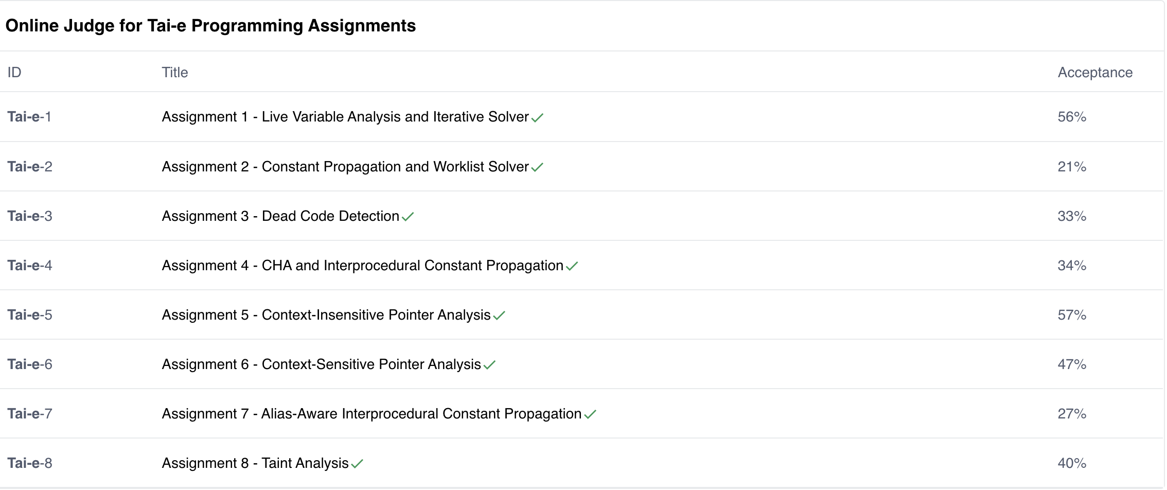
The link of this course is here. I have uploaded my solutions of all assignments, including constant propagation and pointer analysis. They are stored in a git repo. All assignments have passed online judgement and earned full scores.

.

Must and May Analysis

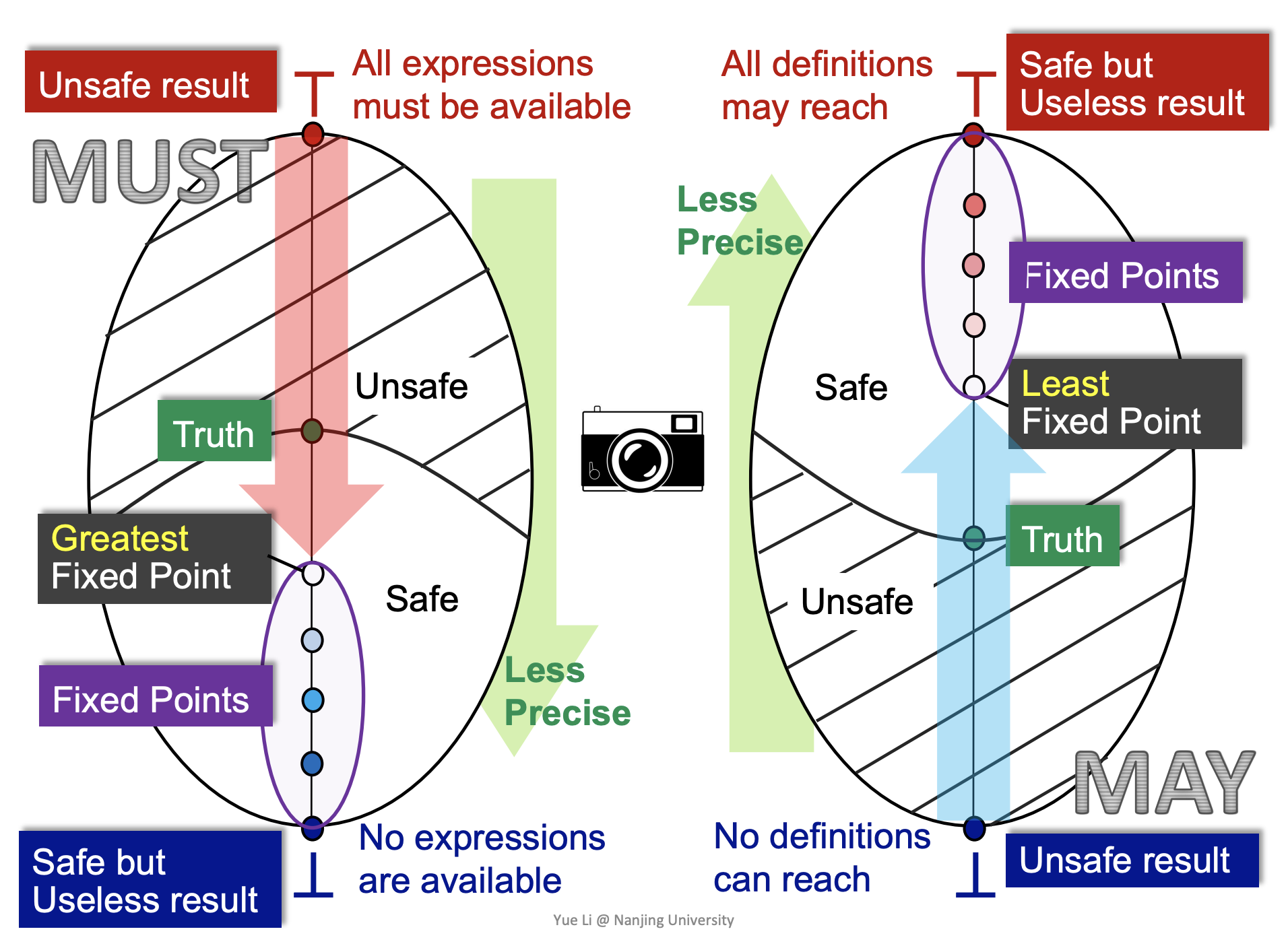
A lattice has greatest and lowest fixed points. Why does must analysis eventually reach to the greatest fixed point and may analysis get to the lowest one?

.

This question actually comes down to propagation direction, where must analysis kicks off from the greatest element of its partial set, and vice versa. Ant analysis flows unsafe facts towards safe facts. A further question is how to identify if the greatest/lowest element holds safe or unsafe facts? I had no idea early but later realize that truthiness is a principal for judgement. When it comes to must analysis, its greatest element represents the meaning that all () must (), and the lowest one shows that none () must (). The content in brackets depends on a question that the analysis answers. From a truthiness perspective, we could kind of feel that the meaning of the greatest element is unsafe because there may be false positives, while that of the lowest one is too safe because many positive facts are excluded and a few of them are left. In order words, the judgement behind “none () must ()” is safe without including any wrong results, but useless. So, we do not want to see our analysis reach there. This also reflects on why we only focus on the greatest fixed point for must analysis even though there are other fixed points available as well.

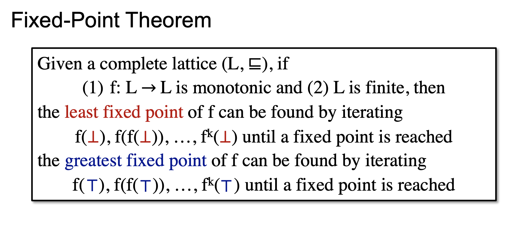
Once we know which element is utilized as a starting point, the kind of the fixed is understood according to fixed-point theorem. If we apply a transfer function to the greatest point, then the fixed point corresponds to be greatest. Furthermore, regarding must analysis, its operator in lattice is meet (intersection), indicating that only true facts are left through propagation, thus the greatest fixed point is the lower bound.

.

Last but not least, a rule of thumb in design of a new analysis approach is soundness even though soundiness has been proposed against unrealistics introduced by soundness in practice. To guarantee soundness, the analysis approach should satisfy over-approximation, and terminate at the point where some true facts are excluded to keep found facts as true in a conservative manner. Therefore, when designing a new analysis approach, we do not just consider monotonicity of a transfer function, but apply over-approximation in the operation of the function.

Upper and Lower bound

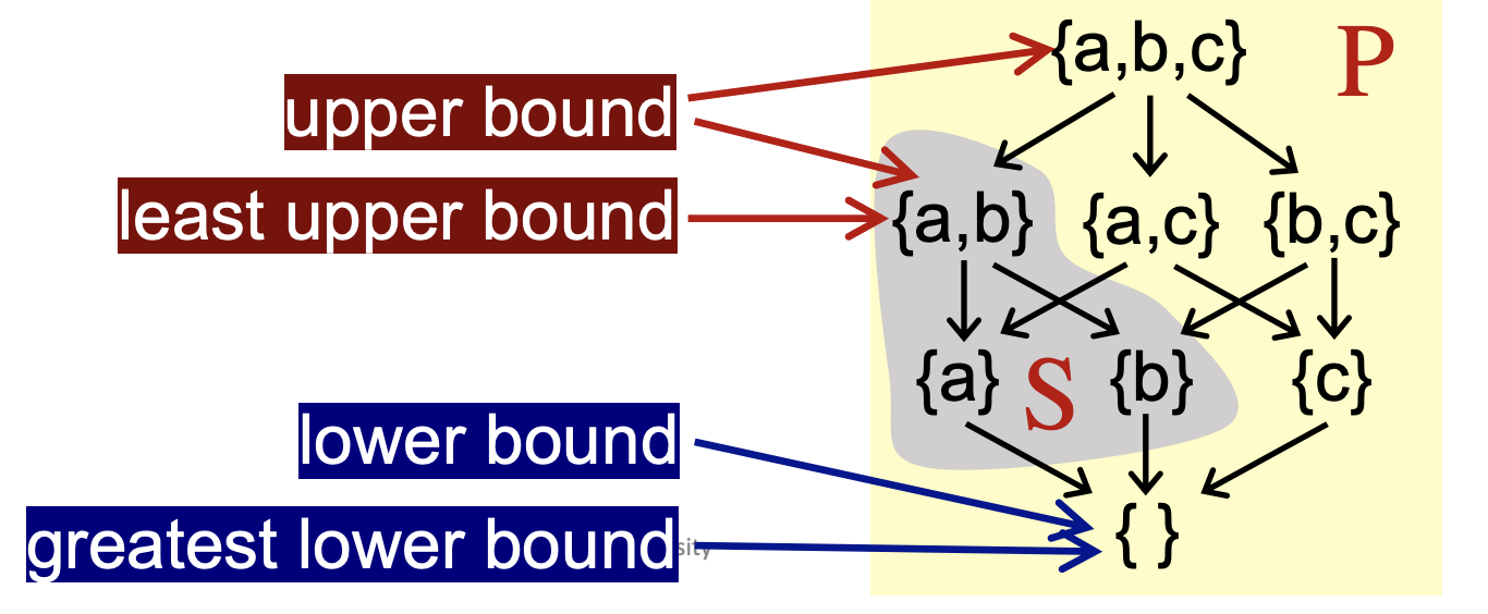
I usually find it difficult to memorize which operation in a partial order set (meet or join) derives a lower or upper bound. Once I have found a figure in slides, I sort of figure out elements in the high position carrying more facts, while those in the low position with less facts.

Basically, when a meet operation is implemented on two elements, data facts of those two will be aggregated in another element that dominates those two in partial order. Hence, when people place this dominant element in the high position, the upper bound is naturally named this way.

.

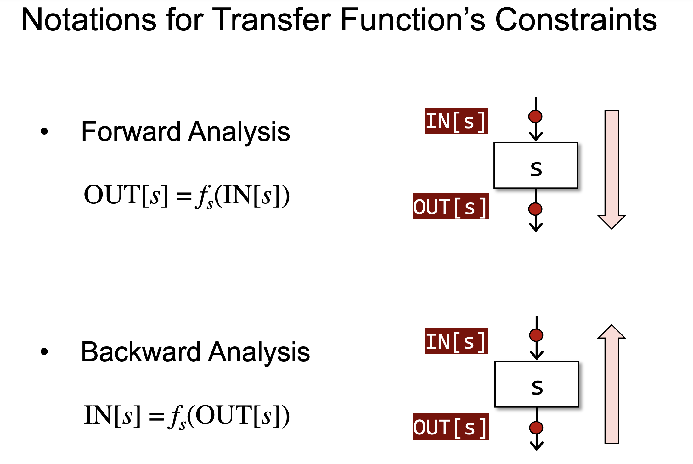
Choice: Forward or Backward Analysis?

Since implementing one assignment about dead code detection, which utilizes live variable analysis and constant propagation, I have sort of figured out the essence of forward and backward analysis. Basically, when we need only one analyse, there is no hard rule in such a choice.

Live variable analysis is a backward analyse aggregating information from an exit point, while constant propagation is a forward analyse, gaining information from a program’s entry. That is to say, whenever we pick up a statement and inspect its IN and OUT fact sets, we could have access to results of those two analyses from two opposite directions. Information from both directions will meet each other along the way and come into play in a situation where we aim at finding a variable definition assigned with a constant which will be used later. For example, with a code snippet as shown below,

int x = 1;
... // any statement without effect on the variable "x"
foo(x);

Finding such a variable will become more cumbersome if we implement both analyses in the same direction - forward or backward, then information about foo(x) cannot be passed back to previous definition statements for analysis.

.

Flow-sensitive vs Flow-insensitive

I haven’t forgotten how much time I spent on Assignment 3, and have a mixed feeling at the end I found all test cases in the online judgement system are way trivial than I thought, even though I do learn a lot about how messy a flow-insensitive design could eventually become. However, it is quite a good mind opener, giving me some insights on when to take on flow-sensitivity or flow-insensitivty.

Assignment 3 asks us to implement a dead code detector, I employed a flow-insensitive algorithm throughout my solution, by dealing with nested statement cases. Although the hidden test cases in the online judgement system do not reach to this level of complexity, I still thought a lot and improved my analyse towards a thorough solution. For example, having a if statement, we are required to combine constant propagation results to identify which branch will not be ever taken. This is all this assignment about, while I am too foolish to consider nested if statements, or a nest of if or switch statements. Thus, a problem to identify the exit point of a switch or if statement comes down to resolving intermediate representation, that requires a lot of considerations on nodes and their in edges to match an exit point to a corresponding statement. Like the next section Abstract Syntax Tree vs Intermediate Representation talking about AST and IR, converting IR back to AST may lose precision in syntax, especially for nested cases. Hence, the most complicated situation is that an if and switch statement is mutually nested, making it pretty hard to measure their scope and to peal one off another; moreover, flow-insensitive processing is global and out of order, that we have no idea about whether an if statement is nested in others, and whether this statement has already been deal with. All those problems contribute a high level of difficulty for a flow-insensitive implementation, thus I may prefer to a flow-sensitive solution that has an advantage of tackling those nested situations.

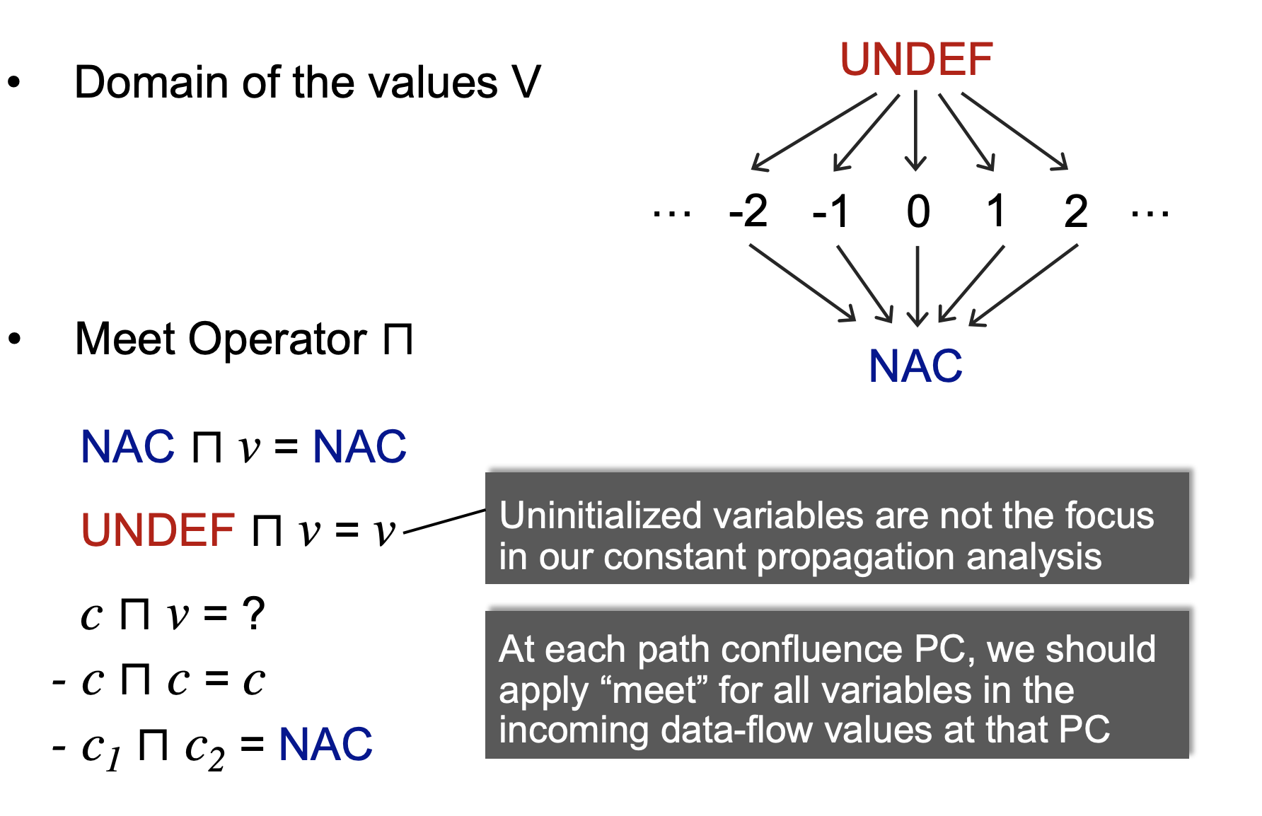
Constant Propagation

At the moment when I am writing down here, I look back constant propagation and fail in figuring out the meaning of top and bottom elements. Since it belongs to must analysis, as of my understanding, the bottom element should represent that none of variable must hold a constant, which sounds unsafe but is wrong. Is there anything or information I miss out on? So, I review its question - “given a variable x at program point p, determine whether x holds a constant at p?”, and then realize that variables need to be defined and initialized before hold a constant. “all vars must hold a constant” could be reduced to a more unsafe level, meaning that all vars are undefined and uninitialized at any program point, and this statement is reflected on the top element. In regards to the bottom one, “none of var must hold a constant” is safe by making any wrong judgement according to the asked question but useless. Its data fact set does not contain any wrong variable that does not hold a constant, thus there is no any false positive, which satisfies completeness. Its lattice preview is like a diamond, which indicates that a defined and initialized variable is able to hold a constant.

.

Constant propagation is considered as crucial and takes up three assignments throughout this course. Especially, the previous assignment is a foundation to the later one, which is well-organized. The first one is a simple one, where students implement it against its algorithm in slides; the second one is more complicated and requires students to implement interprocedural constant propagation, where transition of data facts to a method call needs to be considered; the third one is pretty interesting and more practical, where students are asked to deal with instance field access, array access, and static field access using alias analysis, which works out by using pointer analysis results.

Its applications include compiler optimization, and deal loop detection, etc.

Pointer Analysis

Pointer analysis is a fundamental analyse. This course asks students to implement context-insensitive model, and context-sensitive one. Both of them utilize a flow-insensitive approach, and this eases difficulty of development and represents a clear application logic. The key of this approach is to assume each part of logic has no idea about how other parts are going on, and needs to deal with all cases. For example, when a method is called, it needs to be added in a call graph and connects edges between arguments and its parameters in pointer flow graph, such that a data fact could flow through at some points.

When it comes to context sensitivity, there are three approaches to maintain a context, including callsite, object creation, and type (caller class). The most attractive comparison appears between type and object approaches. Type stands out in terms of performance and effectiveness, it has less call graph edges than object approaches though. More call graph edges are found, more precise this analyse is. Precision has a profound impact on analyses built in pointer analysis, such as alias analysis and tain analysis.

Taint Analysis

Taint analysis shares similar ideas of pointer analysis. That is to say that tainted objects are liquid and flow through pointer flow graph. Additionally, we need to configure source functions, sink functions, and taint transfer in a configuration file. whenever a source function is invoked, a taint object will be created and added into a corresponding var or a field. Taint transfer is better dealt with whenever a new object propagates and a method is called.

Slicing for Taint Value Flow

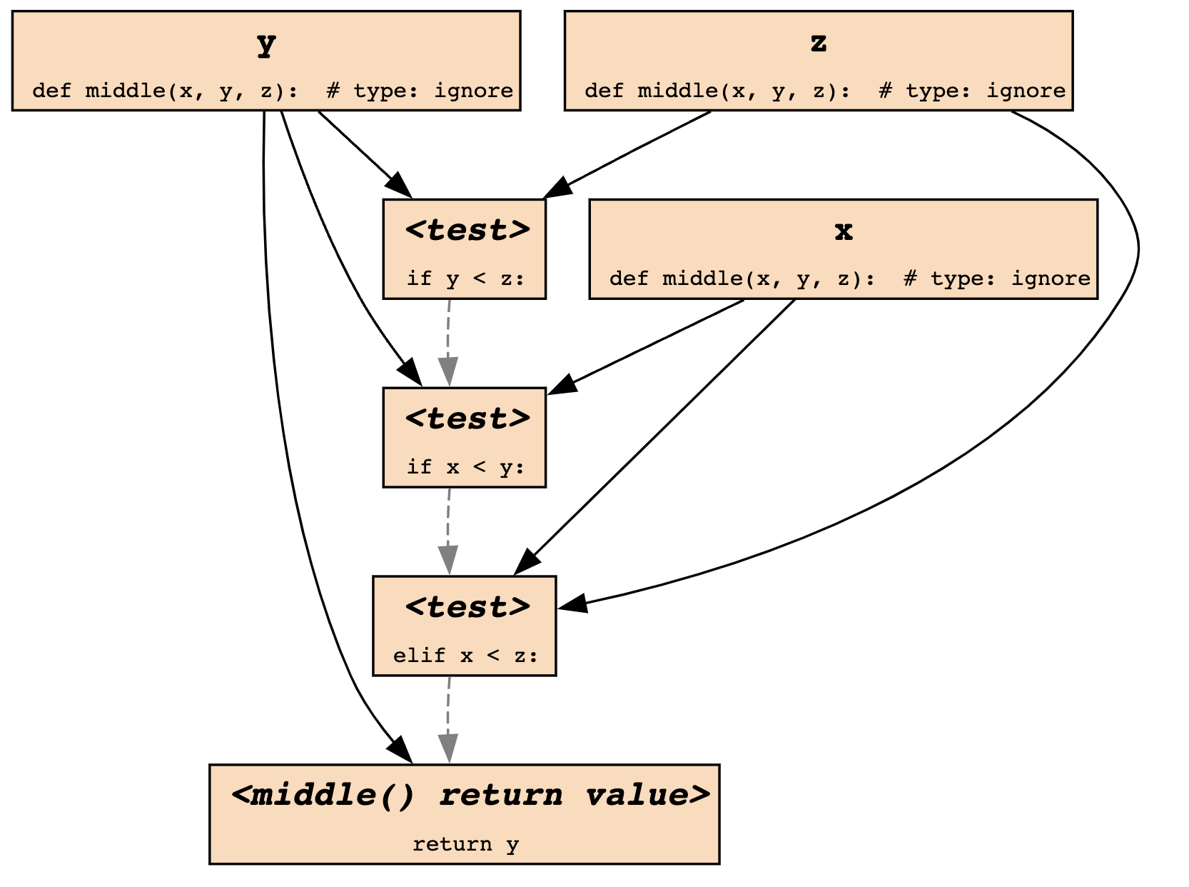
Slicing is a technique, pearing interesting execution paths from a whole program. Specifically, a dependency graph that contains control and data dependencies, is generated statically or dynamically, and is often used to track failure origins. Slicing can be conducted in a forward or backward manner. Both of them are easily understandable, but sort of vague in terms of the actual adaption. I only knew its concept until read the paper sfuzz. The paper aims at identifying vulnerabilities via taint analysis, which derives execution trees. Those trees in turn are dependency graphs. I refer to a diagram from debuggingbook, that has been maintained by Andreas Zeller.

.

Why does this graph contribute to taint analysis? If we only pick over those data points that are actually derived from source functions, then a whole graph turns into taint value flows, which we utilize to confirm if any taint data flows into a sink function. Moreover, a lot of effort in combining graphs of different functions is required.

Backward slicing does the opposite, given a data point, tracking back to its origins. This can be used for POC verification of a certain execution path. Of course, there are other potential, that I haven’t known yet~

Abstract Interpretation

This concept is not intruduced throughout this course, while I intentionally like to complete the learning of static program analysis thoroughly and turn to look into abstract interpretation in other materials.

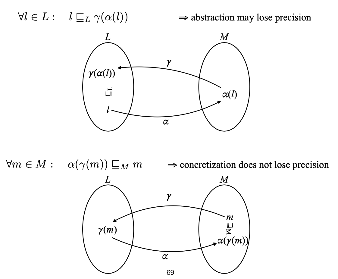
Basically, abstract interpretation aims at removing reduntdant elements of a newly designed analyse relative in the choice of lattice. There are abstract and concrete domains, both of which are complete lattices. abtraction refers to a transition from the a concrete domain to abstract one by a function called abstraction functions, and the flip side is called concretization functions. It is a moment to introduce Galois connection, which holds when these two types of function are monotone and two properties are satisfied:

.

Essentially, the first property related to “extensive” over-approximates a concretization transition over an element in an abstract domain, which results in a concretized element dominating an original element that has been abstracted in the partial order. In a bigger picture, this property compensates missed-out elements accoring to the abstract sementics. When it comes to the second property, that gives the most precise possible abstract description description for any element in the semantic lattice, which is precise than its starting element during this transition.

.

Regarding the top diagram in the figure, the finally concretized element is higher than l, and dominates in the partial order, indicating an extension in lattice. For the bottom one, m dominates the final element, meaning that a reduction is applied in the lattice and the below element is more precise. Essentially, a concrete domain has infinite objects, some of which represent a program property, and what abstract interpretation does is to look for a upper bound that includes those objects and sees the same property, such that we could prove from the point. Otherwise, the only way to prove this property is to enumerate those infinite objects, which is impossible.

Example of An Abstract Domain

I was confused about what an abstract domain really refers to. What is the difference between a concrete and abstract domain? I read through relevant slides and thought that I comprehand it more or less.

The definition of abstract domain includes:

• A domain captures properties of interest
• A partial order that sorts out abstract elements by precision
• Abstract transfer functions that compute on this domain

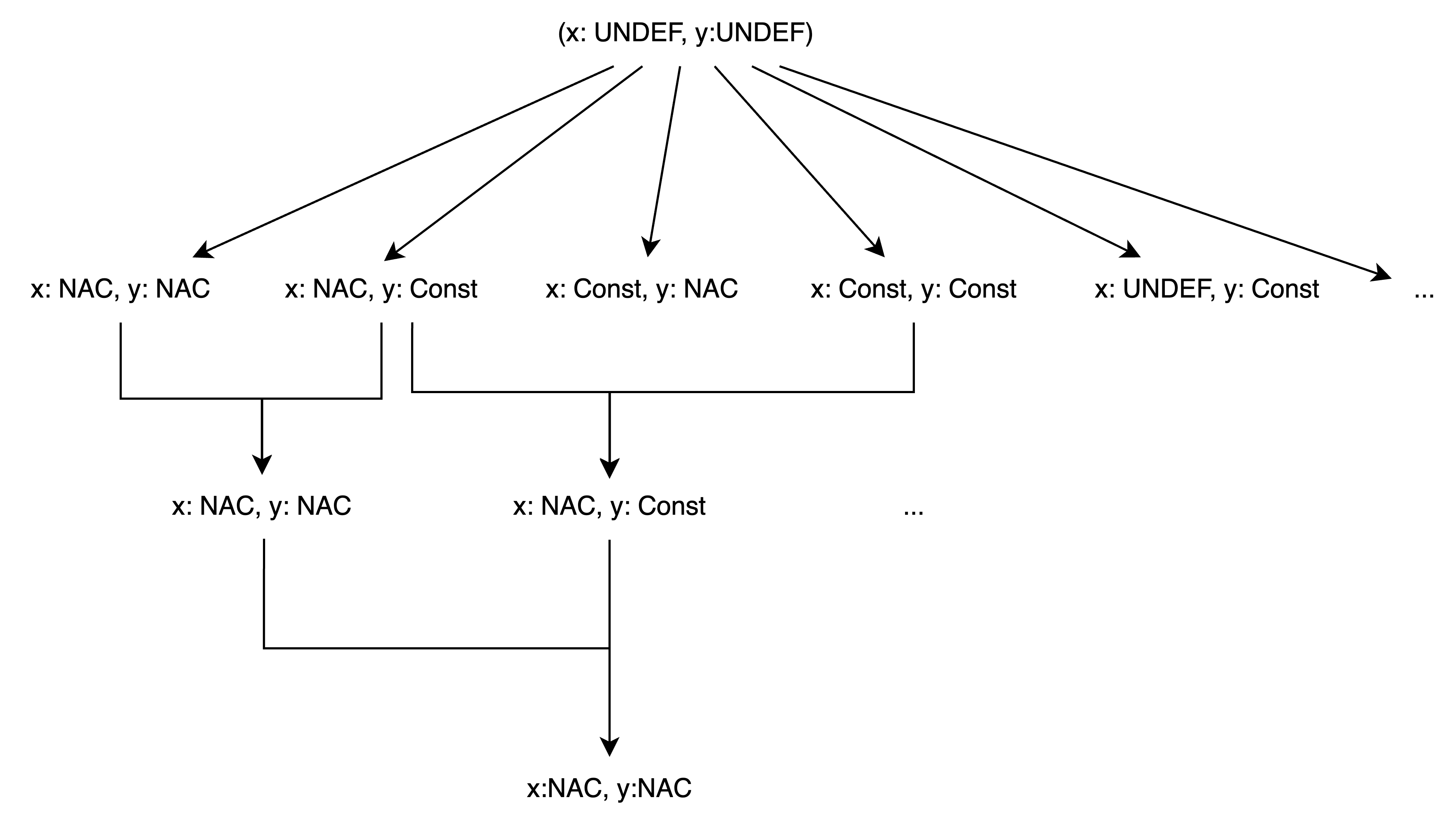
Suppose that we apply those definitions in constant propagation, where a variable is classified into one of those properties, including UNDEF, NAC, and Constant. The first one means that a var holds an integer with 10 or whatever in a concrete domain, but an abstract domain does not focus on its exact value but its property, which is Constant in this case; The second one is vague to me, and I do not think that precision is a key in order, but just a relationship between two elements. Precision, speaking of my experience of implementing pointer analysis, is determined by transfer functions, which make a change in a data fact set and push analysis towards a fixed point. Choosing a good fixed point could avoid losing false negatives for must analysis.

Furthermore, looking for a correct transfer function is hard, and finding the precise one that helps reach out to a good fixed point is even harder. With pointer analysis as an example, its transfer function has to interpret rules for different cases, such as virtual method call, array access. Hence, designing a correct transfer function should be tighted with considerations on those rules. So, those two challenges remain in abstract interpretation.

I draw a diagram to represent an abstract domain of constant propagation.

.

Abstract Syntax Tree vs Intermediate Representation

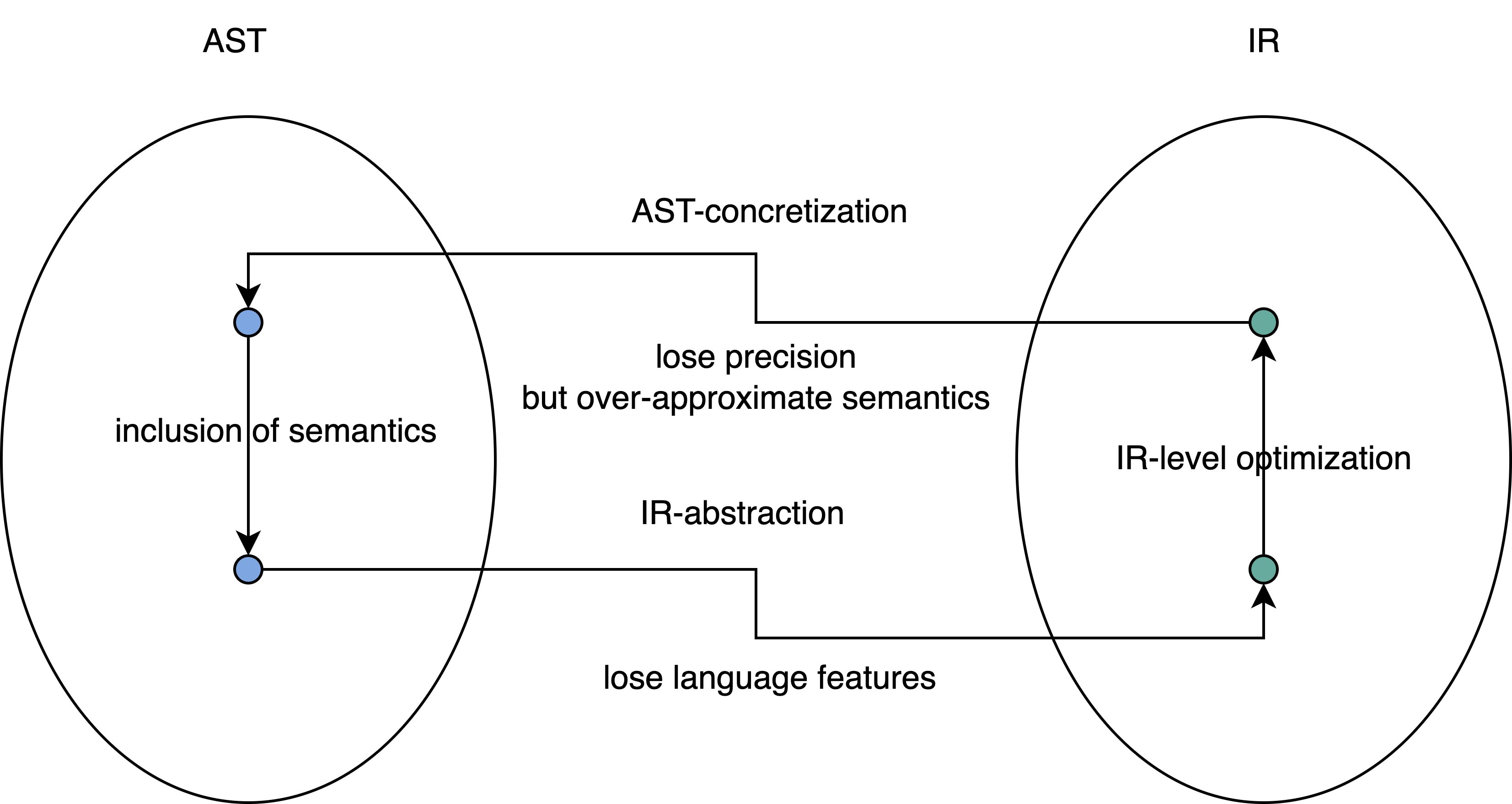
I write down AST and IR here, because I feel like those two concepts are internally connected as concrete and abstract domain could be transfered to each other.

First of all, need to introduce both of them. AST is often language dependent and contains grammer structure. It benefits type-checking, but has non-straighforward control flow information to utilize. In contrast, IR contains control flow information, tosses away language features, and represents in low-level machine code. Hence, without language dependency, it is usually considered as the basis for static analysis.

AST is treated as a concrete domain, and carrys details on a specific language, such as how a do-while loop could be represented in AST.

The abstract syntax tree is flattened as machine code and those language features are lost, leading to a lose in precision, when AST is converted to IR (abstract domain). More interestingly, dealing with IR allows us to design a generalized analyse, which sounds like an abstract operation. Furthermore, IR could be re-compiled back to pesudo code like reverse engineering, which contains more coarse-grained AST information because many temporary variables and mis-interpretation in a language structure could occur, rendering the generated code hardly similar to the original version. What does coarse granularity indicate behind the scene? In essence, re-compilation over-approxiamtes in order to guarantee program correctness, and introduce many in-process variables without losing its original semantics. Moreover, over-approximation may lose precision, but its generated code snippet always includes the semantics of original one which has probably been simplified via a certain level of optimization.

.

Understanding Proof of Properties From Harmonic Series (Mathematics)

Basically, in case that a certain property cannot be easily proven by a set of facts named A, we turn to resort to proof with other facts, e.g., another set of facts B that partially orders A. Let say A ⊆ B in a lattice. Moreover, the set B has advantages in mathematical formalization, which benefits us from proving the property. Abstract interpretation could convert the set A into that of an abstract domains via abstract functions, which in turn is converted back to the previous concrete domain via concretization functions. The newly concretized set is B, for which the property is proven and holds. Thus, the property also holds for A according to their relationship in partial order.

Harmonic Series shares the similar idea. Having the following series,

we want to prove a property that it is a divergent series, where the values of these partial sums grow arbitrarily large. However, it is quite obvious that we cannot sort out those numbers somehow. So, what people do is to “downgrade” those numbers, which we could see as one round of abstraction and concretization. Those new numbers are smaller than previous ones, but they embody some similarities to allow gathering of same numbers, such that two 1/4 could sum up to 1/2, and four 1/8 could add up to 1/2 as well, thus we eventually prove that we have infinite 1/2 and the series will grow arbitrarily large.

Regardless of whether this equotion could form a lattice, it is very clear that the new numbers and old ones respect a relationship in partial order, and divergence holds for both. We could gain some insights on the connection between abstract interpretation and math.

Static vs Dynamic Analysis

Static analysis that follows over-approximation will not miss any bugs but may generate false positives (in such a case, we need to adjust abstraction). In contrast, dynamic analysis facilitates under approximation and picks a piece of execution path to be analyzed. Its advantages mainfest in not generating false positives, but missing out on some bugs. Hence, those two approaches are complementary.

My research interests lie at firmware re-hosting and program testing. Basically, emulation is an over-approximation approach to running the target program with all possible states. Hardware-in-the-loop is another approach without considerations on hardware dependency. Firmware binary runs on its own MCU, and analysts get access to its execution states via debugging interfaces, such as JTAG. Then they aggregate those information to analyze where potential bugs or vulnerabilities may appear.

Frankly, I personally have a strong preference to static analysis mainly because dynamic analysis introduces uncertainties due to its under approximation. Thus, many cutting edge research work based on this approach intentionally claims their practicality and usability for industries. It sounds reasonable to apply this approach epsecially when no new theories are found in program analysis. An attempt to combine both of them is a good practice as well.

Symbolic and Concolic Execution

TODO